AN UPDATED VERSION OF THIS TUTORIAL IS AVAILABLE HERE
This post is a brief tutorial about how to perform the accuracy assessment of a land cover classification using the Semi-Automatic Classification Plugin (SCP) for QGIS.
In particular, we are going to create ROIs using random points over the image (a new function of SCP 3.1.0), which will be photo-interpreted and used as reference for the accuracy assessment.
This tutorial assumes that we have already performed the classification of a Landsat image following the instructions of this previous tutorial. The land cover classes of this classification are:
- Class 1 = Water (e.g. surface water);
- Class 2 = Vegetation (e.g. grassland or trees);
- Class 3 = Built-up (e.g. artificial areas, buildings and asphalt);
- Class 4 = Bare soil (e.g. soil without vegetation).
The following are the main phases:
- Automatic creation of ROIs at random points;
- Photo-interpretation of created ROIs;
- Calculation of classification accuracy using created ROIs as reference.
First download the Landsat 8 image from here (data available from the U.S. Geological Survey), the training shapefile and spectral signature list. Also, download the final classification that we are going to assess.
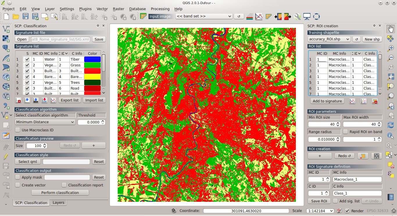
Following the instructions from my previous tutorial, convert raster bands from DN to Reflectance and create the band set, load the training ROIs and the spectral signatures, as well as the land cover classification. This image shows you the starting point of this tutorial.

1. Automatic creation of ROIs at random points
We are going to create random points over the image. SCP allows for the calculation of point coordinates randomly distributed over the area of the Input image. In addition, it is possible to create a number of points distributed inside each cell of a grid with a defined size, or define a minimum distance between points.
Steps:
- Create a new training shapefile clicking the button New shp in the ROI creation dock (e.g. accuracy_ROI.shp);
- Open the tab Multiple ROI creation by clicking the button
 in the ROI creation dock; beside Number of random points type 25 that will be single pixels ROIs;
 - The ROI creation parameters are set according to the ROI parameters in the ROI creation dock; in order to have 1 pixel ROIs set both Min ROI size and Max ROI width to 1;

- Now in the tab Multiple ROI creation click Create random points; a list of random X, Y coordinates will be added to the table;

- Suppose we want also 25 ROIs up to 40 pixel size; in the ROI creation dock set both Min ROI size and Max ROI width to 40 (it is also possible to change the other ROI creation parameters according to your needs);
- In the tab Multiple ROI creation check minimum point distance and set the value to 1700 (in meters), in order to avoid overlapping ROIs; then click Create random points; also, uncheck the checkbox Add sig. list because we do not need spectral signatures;

- Now we can create the ROIs; click the button Create and save ROIs; after a while, created ROIs will be listed in the ROI list.
Attention! Setting a minimum distance between points can produce fewer points than the number defined in Number of random points
2. Photo-interpretation of created ROIs
As you can see, all the created ROIs have the same MC ID (i.e. macroclass ID) and C ID (i.e. class ID); using the SCP interface it is easy to assign the correct class to each ROI with photo-interpretation (for this purpose, a useful plugin is OpenLayers which allows for the display of high resolution data in QGIS). During the photo-interpretation, one can use different color composites for identifying the various classes.
Steps:
- Double click on the first ROI in the ROI creation dock in order to zoom to the ROI over the Landsat image;
- Classify the ROI MC ID and C ID with a click on the corresponding field in the ROI list; we can classify just the MC ID because the classification we are going to assess was classified using the MC ID (the definition of MC Info and C Info is not required for the accuracy assessment, although it can be useful).

- Water (e.g. surface water): MC ID = 1
- Vegetation (e.g. grassland or trees): MC ID = 2
- Built-up (e.g. artificial areas, buildings and asphalt): MC ID = 3
- Bare soil (e.g. soil without vegetation): MC ID = 4
The following are a few examples of ROIs.
 |
| ROI over bare soil |
 |
| ROI over vegetation |
You can download the accuracy ROIs from here.
3. Calculation of classification accuracy using created ROIs as reference
The accuracy assessment is performed by comparing the ROIs and the classification. The result is an error matrix and a error raster that shows the errors in the map (where each value is a class of comparison between classification and reference shapefile).
Steps:
- In the Classification dock check Use Macroclass ID, because we use the MC ID field for assessing the classification;
- Select the tab Post processing > Accuracy of the SCP main interface;
- Select classification.tif beside Select the classification to assess and select the accuracy_ROI shapefile beside Select the reference shapefile;

- Click the button Calculate error matrix and select a directory where the error matrix (i.e. a .csv file separated by tab) and the error raster are saved; the error matrix will be displayed, and the error raster will be loaded in QGIS.

The following are the results of the accuracy assessment. Here you can download the error matrix and the error raster.
| ERROR MATRIX (pixels) | Reference | ||||
| Classification | 1 | 2 | 3 | 4 | Total |
| 1 | 1 | 0 | 0 | 0 | 1 |
| 2 | 0 | 71 | 2 | 3 | 76 |
| 3 | 0 | 5 | 52 | 2 | 59 |
| 4 | 0 | 0 | 1 | 32 | 33 |
| Total | 1 | 76 | 55 | 37 | 169 |
Overall accuracy [%] = 92.3
- Class 1: producer accuracy [%] = 100.0; user accuracy [%] = 100.0
- Class 2: producer accuracy [%] = 93.4; user accuracy [%] = 93.4
- Class 3: producer accuracy [%] = 94.5; user accuracy [%] = 88.1
- Class 4: producer accuracy [%] = 86.5; user accuracy [%] = 97.0
The main advantage of this method is that we can assess the accuracy over homogeneous surfaces defined with automatic ROI creation, and not only on single points. It is worth highlighting that Landsat resolution (i.e. 30m) implies mixed pixels (i.e. pixels made of multiple materials at ground), and this must be considered during the photo-interpretation of ROIs assigning the most prevalent class in the pixel area.
Finally, the error of photo-interpretation should be considered, which can affect the accuracy assessment.
Finally, the error of photo-interpretation should be considered, which can affect the accuracy assessment.
If you have questions or thoughts please share them with the Facebook group or the Google+ Community of the Semi-Automatic Classification Plugin for QGIS.